Motif recognition
Time-series sometimes present repeating motifs (or patterns) that are worthwhile identifying. The detection of such motifs can be difficult depending on the amount of noise in the time-series.
In the case of categorical time-series, the lack of a proper metric to measure distance between motifs can make their detection tricky. Improper distances like the number of differences between the two motifs is commonly used.
This package proposes a detection algorithm based on JEREMY BUHLER and MARTIN TOMPA's paper "Finding Motifs Using Random Projections". This algorithm although very precise is not exact. Therefore, when you are done detecting potential motifs with the detect_motifs function, you can refine your results with find_motifs for an exact search.
The main functions return instances of a class called pattern:
pattern — Class
A class storing useful information about found motifs in a time-series. An array of pattern instances is returned when the searching algorithm is done running.
Attributes:
- shape (Array{Any,1}): Array containing the shape (or contour) of the first found repetition of the motif.
- instances (Array{Array{Any,1},1}): all the different shapes from the motif's repetitions, they can vary a bit from one to the next.
- positions (Array{Int,1}): the positions at which the different repetitions of the motif were found.
Main functions
detect_motifs — Function
detect_motifs(ts, w, d, t = w - d; iters = 1000, tolerance = 0.95)
Detects all motifs of length 'w' occuring more often than chance, being identical to each other up to 'd' differences inside of input time-series 'ts'.
Returns an array of pattern, inside of which the patterns are classified by how frequently they are observed. The first elements is therefore the most frequently observed motif, and so on.
Parameters:
- ts (Array{Any,1}): input time-series in which motifs are searched for.
- w (Int): length of motifs to look for.
- d (Int): allowed errors (differences) between motifs repetitions.
- t = w - d (Int): size of the masks to use for random projection in the detection (defaults to w - d).
- iters = 1000 (Int): the numbers of iterations for the random projection process (defaults to 1000)
- tolerance = 0.95 (Float): threshold of motif identification. If set to 1, only matrix entries that are strictly superior to the (probabilistic) threshold are taken into account. Defaults to 0.7, meaning that matrix entries need to be bigger than 0.7*threshold.
Returns :
- motifs : list of
patterninstances sorted by frequency of occurence. motifs[1] is therefore the most frequent motif, motifs[2] the second most observed and so on.
find_motifs — Function
find_motifs(ts, shape, d)
Given a motif of shape 'shape' (array{any,1}), looks for all the repetitions of it which differ only up to 'd' differences inside of the input time-series 'ts'. Input:
Parameters:
- ts (Array{Any,1}) : time-series in which to look for motifs
- shape (Array{Any,1}): shape (aray{any,1}) of the motif to look for.
- d (Int): allowed errors (differences) between motifs
- Returns :
- motif : an instance of
patterncontaining the found repetition of the input 'shape'.
Plotting
To help visualize results, two simple plotting functions are provided.
plot_motif — Function
plot_motif(m::pattern)
Plots all repetitions of an input pattern instance on top of each other to see how similar they are to each other.
Parameters:
- m : Instance of the
patternclass
plot_motif — Function
plot_motif(m::pattern, ts)
Plots all repetitions of an input pattern instance on top of the input time-series 'ts' to better visualize their repartition in time.
Parameters:
- m : Instance of the
patternclass- ts (Array{Any,1}): Input time-series
Example
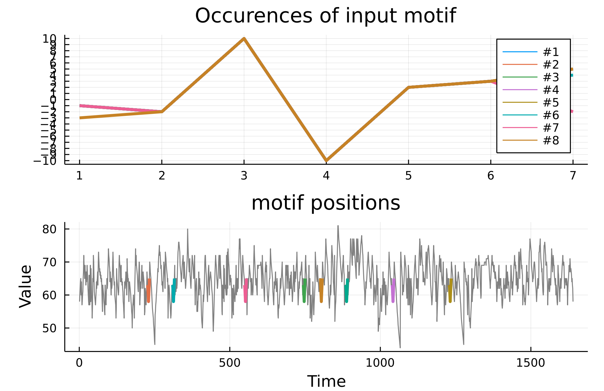
From Michael Brecker's improvisation over the piece "confirmation", we extract a time-series of pitch intervals (difference from one note to the next). A spectral envelope analysis reveals a peak at period 6~7, so we look for motifs of length 7 and allow for 1 error between them. After detection, we visualize the most frequent motif:
using DelimitedFiles
using CategoricalTimeSeries

data_path = joinpath(dirname(dirname(pathof(CategoricalTimeSeries))), "test", "confirmation")
data = readdlm(data_path)
pitch = mod.(data, 12) #Removing octave position: not needed
intervals = pitch[2:end] .- pitch[1:end-1] #getting interval time-series.
m = detect_motifs(intervals, 7, 1; iters = 700, tolerance = 0.7)
plot_motif(m[1]) #plotting most frequent motif

We notice that the motif [-1, -2, 10, -10, 2, 3, 5] seems to be the underlying (consensus) shape. In musical notation, this motif would look like this (written in C major):

We do an exact search with 1 error allowed to check if our previous detection missed any repetitions, and plot the found motif on top of each other:
consensus_shape = [-1, -2, 10, -10, 2, 3, 5]
motif = find_motifs(intervals, consensus_shape, 1)
plot_motif(motif)
Here, we obtain the same plot as before but this is not necessarily always the case. Knowing the consensus motif usually allows to find its repetitions more efficiently.
Now, we visualize the repetitions of the motif in the time-series:
plot_motif(motif, data)