Information bottleneck
The information bottleneck (IB) concept can be used in the context of categorical data analysis to do clustering, or in other words, to look for categories which have equivalent functions.
Given a time-series, the IB looks for a concise representation of the data that preserves as much meaningful information as possible. In a sense, it is a lossy compression algorithm. The information to preserve can be seen as the ability to make predictions: given a specific context, how much of what is coming next can we predict ?
The goal of this algorithm is to cluster categorical data while preserving predictive power.
To learn more about the information bottleneck you can look at [1] or [2]
Quick start
To do a simple IB clustering of a categorical time series, the first step is to instantiate an IB model. Then optimize it via the IB_optimize! function to obtain to obtain the optimal parameters.
data = readdlm("/path/to/data/")
model = IB(data) #you can call IB(x, beta). beta is a real number that controls the amount of compression.
IB_optimize!(model)
The data needs to be presented as a 1-D array, otherwise IB interprets it as a probability distribution (see below).
To see the results, you can use:
print_results(model)
Rows are clusters and columns correspond to the input categories. The result is the probability p(t|x) of a category belonging to a given cluster. Since most of the probabilities are very low, print_results sets every p(t|x) > 0.1 to 1. p(t|x) < 0.1 are set to 0 otherwise for ease of readability (see further usage for more options).
The optimized parameters may vary from one optimization to the next as the algorithm is not deterministic, to obtain global optima, use the search_optima function (see below).
Further usage
To have a better grasp of the results produced by IB clustering, it is important to understand the parameters influencing the algorithm of IB model structures. The two most important parameters are the amount compression and the definition of the context. They are provided upon instanciation:
IB — Type
IB(x, y, β = 100, algorithm = "IB")
IB(x, β = 100, algorithm = "IB")
IB(pxy::Array{Float64,2}, β = 100, algorithm = "IB")
Parameters:
- x (Array{Int,1} or Array{Float,1}): 1-D Array containing input categorical time-series.
- y (Array{Any,1}): Context used for data compression. If not provided, defaults to "next element", meaning for each element of x, y represent the next element in the series. This means that the IB model will try to preserve as much information between 'x' and it's next element. (see
get_yfunction)- β (Int): parameter controlling the degree of compression. The smaller
βis, the more compression. The higherβ, the bigger the mutual information I(X;T) between the final clusters and original categories is. There are two undesirable situations: ifβis too small, maximal compression is achieved and all information is lost. Ifβis too high, there is no compression.
with "IB" algorithm, a highβvalue (~200) is a good starting point. With "DIB" algorithm,β> ~5 can already be too high to achieve any compression.
βvalues > ~1000 break optimization because all metrics are effectively 0.- algorithm (String): The kind of compression algorithm to use. "IB" choses the original IB algorithm (Tishby, 1999) which does soft clustering, "DIB" choses the deterministic IB algorithm (DJ Strouse, 2016) doing hard clustering. The former seems to produce more meaningfull clustering. Defaults to "IB".
- pxy (Array{Float,2}): joint probability of element 'x' to occur with context 'y'. If not provided, is computed automatically. From
xandy.Returns: instance of the
IBmutable struct.
get_y — Function
get_y(data, type = "nn")
Defines and return the context associated with the input time-series data.
Parameters:
- data (Array{Any,1}): 1-D Array containing input categorical time-series.
- type (String): type of context to use. Possible values are "nn" or "an". Defaults to "nn" (for next neighbor). This means, if data = ["a","b","c","a","b"], the "nn" context vector y is ["b","c","a","b"]. Chosing "an" (for adjacent neighbors) not only includes the next neighbor but also the previous neighbor, every element of y is then a tuple of previous and next neighbor.
Returns:
y, associated context todata.
Additional functions
calc_metrics — Function
calc_metrics(model::IB)
Computes the different metrics (H(T), I(X;T), I(Y;T) and L) of an IB model based on its internal probability distributions.
Parameters:
- model: an IB model
Returns: (ht, ixt, iyt, L), metrics. ht is the entropy of the clustered representation. ixt is the mutual information between input data and clustered representation. iyt is the mutual information between context and clustered representation. L is the loss function.
search_optima — Function
search_optima!(model::IB, n_iter = 10000)
Optimization is not 100% guaranteed to converge to a global maxima. this function initializes and optimizes the provided IB model n_iter times, then, the optimization with the lowest L value is selected. The provided IB is updated in place.
Parameters:
- model: an IB model
- n_iter (Int): defined how many initialization/optimization are performed for the optima search.
Returns:
nothing. The update is done in place.
print_results — Function
print_results(m::IB, disp_thres = 0.1)
Displays the results of an optimized IB model.
Parameters:
- m: an IB optimized model
- disp_thres (Float): The probability threshold to consider that a category belongs to a given threshold. This makes reading the results more easy. Defaults to 0.1.
Returns:
nothing. Print the results.
If you want to get the raw probabilities p(t|x) after optimization (print_results filters it for ease of readability), you can access them with :
pt_x = model.qt_x
Similarly, you can also get p(y|t) or p(t) with model.qy_t and model.qt.
get_IB_curve — Function
`get_IB_curve(m::IB, start = 0.1, stop = 400, step = 0.05; glob = false)`
Scans the IB plane with various values of beta to get the optimal curve in the IB plane.
Parameters:
- m: an IB optimized model
- start (Float): The start β value.
- stop (Float): The ending β value
- step (Float): The steps in β values that the function takes upon optimizing the provided model.
- glob (Bool: if True, each optimization is done with the help of
search_optima(more computationally demanding). Default to False.Returns: (ixt, iyt) the values of mutual information between data and clusters and context and clusters for each β value used by the function.
Examples
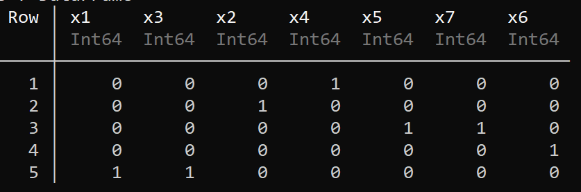
Here is a concrete example with data from Bach chorales. The input categories are the 7 types of diatonic chords described in classical music theory. In this case, the data (input series and context) have already been compiled into a co-occurence table, so we instantiate the IB model with a probability distribution:
using CategoricalTimeSeries
using CSV, DataFrames

data_path = joinpath(dirname(dirname(pathof(CategoricalTimeSeries))), "test", "bach_histogram")
bach = DataFrame(CSV.File(data_path))
pxy = Matrix(bach)./sum(Matrix(bach)) #normalizing the co-occurence table to have probabilities.
model = IB(pxy, 20) #instantiating the model with co-occurence probabilities.
search_optima!(model, 1000)
print_results(model)
The output is in accordance with western music theory, but reveals interesting features. It tells us that we can group category 1, 3: this corresponds to the tonic function in classical harmony. Category 5 and 7 are joined: this is the dominant function. Interestingly, category 2 and 4 (subdominant function) have not been clustered together, revealing that they are not used in a totally equivalent fashion in Bach's chorales.
In the next example, we instantiate the model with a time-series (saxophone solo) and define our own context.
using CategoricalTimeSeries
using CSV, DataFrames

data_path = joinpath(dirname(dirname(pathof(CategoricalTimeSeries))), "test", "coltrane_afro_blue")
data = DataFrame(CSV.File(data_path))[!,1]  #time-series of notes from saxophone solo (John Coltrane).
context = get_y(data, "an") # "an" stands for adjacent neighbors.
model = IB(data, context, 500) # giving the context as input during instantiation.
IB_optimize!(model)
Now, we show how to plot the IB curve:
using Plots, CSV, DataFrames
using CategoricalTimeSeries

data_path = joinpath(dirname(dirname(pathof(CategoricalTimeSeries))), "test", "bach_histogram")
bach = DataFrame(CSV.File(data_path))
pxy = Matrix(bach)./sum(Matrix(bach)) #normalizing the co-occurence table to have probabilities.
model = IB(pxy, 1000) #instantiating the model with co-occurence probabilities.
x, y = get_IB_curve(model)
a = plot(x, y, color = "black", linewidth = 2, label = "Optimal IB curve", title = "Optimal IB curve \n Bach's chorale dataset")
scatter!(a, x, y, color = "black", markersize = 1.7, xlabel = "I(X;T) \n", ylabel = "- \n I(Y;T)", label = "", legend = :topleft)

Acknowledgments
Special thanks to Nori Jacoby from whom I learned a lot on the subject. The IB part of this code was tested with his data and reproduces his results.
The present implementation is adapted from DJ Strouse's paper https://arxiv.org/abs/1604.00268 and his python implementation.